Logistic Regression

Given an input feature vector \(\vec{x}\) maybe corresponding to an image that you want to recognize as either a cat picture or not a cat picture, you want an algorithm that can output a prediction, which we'll call \(\hat{y}\). which is your estimate of \(\vec{y}\).

So, Given \( \vec{x} \), we can define that  \( \vec{\hat{y}} = P(y=1 | \vec{x})\). Thus, we could try to define the estimate function as \( \hat{y} = w^{T} x + b \) but, since \(\hat{y}\) must be \( 0 \to \hat{y} \to 1 \). that is why we are going to use the following definition:

\[  \hat{y} = \sigma(w^{T} x + b) \] 

Where \( \sigma(z) = \frac{1}{1+e^{-z}} \) , if  \( z \to \infty, \quad \sigma \to 0 \)  while,   \( z \to -\infty, \quad \sigma \to 1 \) 

Cost Function

To train the parameters \( w \) and \( b \) of the logistic regression model. you need to define a cost function, let's take a look at the cost function.

Give training set \(\{ (x^{(1)}, y^{(1)}), \ldots, (x^{(m)}, y^{(m)}) \}\) of \( m \) samples, and wants \( \hat{y}^{i} \approx y^{i} \). We need to define a Loss Function for this problem as:

\[ \mathscr{L} (\hat{y}, y) = -[ y \log \hat{y} + (1-y) \log (1-\hat{y}) ] \]
Note that the loss function is a measure of how you are doing on a single training sample.

Loss function justification:

• If \( y=1\) :  \( \mathscr{L} = - \log \hat{y} \)  so you want \( \log \hat{y} \) to be large, then want \( \hat{y} \) LARGE.
• If \( y=0\) :  \( \mathscr{L} = - \log (1-\hat{y}) \) so you want \( \log (1-\hat{y}) \)  to be large, then want  \( \hat{y} \) SMALL.

So, the cost function (logistic regression performance on the entire training set) would be defined as:

\[ J(w, b) = \frac{1}{m} \sum_{i=1}^{m}  \mathscr{L}   (\hat{y}, y)  =  \frac{-1}{m} \sum_{i=1}^{m} [  y^{(i)} \log \hat{y}^{(i)}  + (1-y^{(i)} ) \log (1-\hat{y}^{(i)} )  ]  \]

Note: \(\log_e x \equiv \ln x \equiv \log x\)

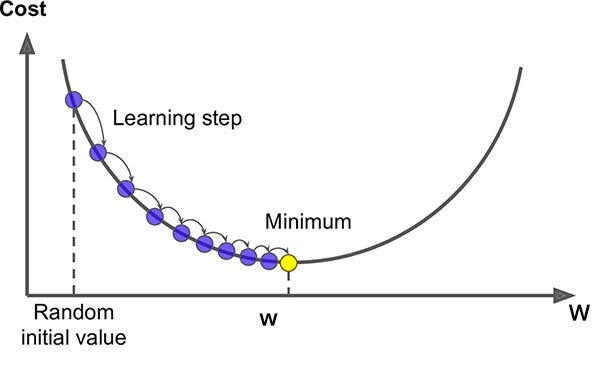
Gradient Descent

Simply, we want to find the weights \( w, b \) that minimize the Cost function \( J(w, b) \). Then, we would take the derivative of the cost function w.r.t \( w \) which we will call \( dw = \frac{\partial J}{\partial w} \). same applies to \( da \).

Then, we repeatedly do the following updates:

• \( w := w - \alpha dw \) 
• \( a := a - \alpha da \) 

where \( \alpha \) is the "learning rate" which define how large the step size we took in one update iteration.

So, when the slope is positive you will subtract from e.g. \( w \) the amount \( \alpha dw \) so that you move \( w \) toward the global minima and vice versa.

Logistic Regression Gradient Descent

Recap

• \( z = w^{T}x + b \)
• \( \hat{y} = a = \sigma(z) \)
•  \( \mathscr{L} (a, y) = -[ y \log a + (1-y) \log (1-a) ] \)

Then, Inputs are \( x_1, w_1, x_2, w_2, b   \to  a = \sigma(z) \to  \mathscr{L} (a, y)  \) 

Derivatives

let \( da = \partial{ \mathscr{L} } / \partial{a} \) which will be \( da = \frac{-y}{a} + \frac{1-y}{1-a} \) . And let \( dz = \partial \mathscr{L} / \partial{z} \).
\( \because \partial \mathscr{L} / \partial{z}  = (  \partial \mathscr{L} / \partial{a} ) (\partial{a} / \partial{z} ) \) (chain rule).
\( \because a = \sigma(z) \) and \(  \because   e^{-z} = \frac{1}{a} - 1 \)
\( \therefore  \partial{a} / \partial{z}  = e^{-z} / (1+e^{-z})^2 = ( \frac{1}{a} - 1 ) / ( 1 + \frac{1}{a} -1 ) ^2  = a(1-a)  \) 
\( \therefore dz =  da * a(1-a) = a - y \) also note that \( db = dz * (\partial{z} / \partial{b}) \therefore db = dz \)
Finally, \( \frac{\partial{\mathscr{L}}}{\partial{w_i}} = dw_i = dz * (\partial{z} / \partial{dw_i}) \to dw_i = dz * x_i \)

Then, Update Step shall be

• \( w_1 := w_1 - \alpha dw_1 \)
• \( w_2 := w_2 - \alpha dw_2 \)
• \( db := db - \alpha db \)

Note that this analysis was just for one input sample. but, for \( m \) training samples:
\[ \frac{\partial{J}}{\partial{w_j}} = \frac{\partial{J(w,b)}}{\partial{w_j}} = \frac{1}{m} \sum_{i=1}^{m}  \frac{\mathscr{L} (a^i, y^i)}{\partial{w_j}}  \] 

Non-Vectorized Logistic Regression

Initialize the following variables: \(  J = 0,\quad dw_1 = 0,\quad dw_2 = 0,\quad db = 0  \)

\(
\begin{aligned}
&\textbf{for } i = 1 \text{ to } m: \\
&\qquad z^{(i)} = w^T x^{(i)} + b \\
&\qquad a^{(i)} = \sigma(z^{(i)}) \\
&\qquad J \mathrel{+}= - \left[ y^{(i)} \log a^{(i)} + (1 - y^{(i)}) \log (1 - a^{(i)}) \right] \\
&\qquad dz^{(i)} = a^{(i)} - y^{(i)} \\
&\qquad dw_1 \mathrel{+}= x_1^{(i)} dz^{(i)} \\
&\qquad dw_2 \mathrel{+}= x_2^{(i)} dz^{(i)} \\
&\qquad db \mathrel{+}= dz^{(i)} \\
\end{aligned}
\)

Finally, \(  J = \frac{J}{m},\quad dw_1 = \frac{dw_1}{m},\quad dw_2 = \frac{dw_2}{m},\quad db = \frac{db}{m}  \)

Vectorize \( dw \) for \(n_x\) features input

Instead of \(   dw_1 = 0,\quad dw_2 = 0 \) defne \( dw = np.zeros((n_x, 1)) \)
Then, for each training sample \(i\) do  \( dw += X^{(i)} dz^{(i)} \), and finally average by the count of the training samples \( dw /= m \)

Vectorizing Logistic Regression

For \( m = 3 \) training samples we need to calculate forward propagation as follows:

\[
\begin{aligned}
z^{(1)} &= w^T x^{(1)} + b &\quad& a^{(1)} = \sigma(z^{(1)}) \\
z^{(2)} &= w^T x^{(2)} + b &\quad& a^{(2)} = \sigma(z^{(2)}) \\
z^{(3)} &= w^T x^{(3)} + b &\quad& a^{(3)} = \sigma(z^{(3)})
\end{aligned}
\]

But, because \( x^{(i)} \) is \( (n_x x 1) \) let \( w \) be the same dimensions. 
 \[ \because X = \begin{bmatrix}
\vdots &  \vdots   &  \vdots   &  \vdots   \\
x^{(1)}  & x^{(2)}  & \cdots & x^{(m)}  \\
\vdots &  \vdots   &  \vdots   &  \vdots 
\end{bmatrix} , \qquad \therefore [ z^{(1)} z^ {(2)}  ... ]_{1xm} = W^T X_{nxm} + b_{1xm}
\] 

And Using Python we can simply apply this calculation as follows:

import numpy as np
z = np.dot(w.T, X) + b 

"""
n: features, m: training samples 
z is vector (1xm)  
w is matrix (nxm)
b is scaler (1x1) "broadcasting" into vector of correct dimensions. """ 

Also, \( \because  A = [ a^1  a^2 \cdots a^m ] = \sigma(z) \)  
And for \( m \) samples \( \to dz^{(1)} = a^{(1)} - y^{(1)} , \quad  dz^{(1)} = a^{(1)} - y^{(1)} , \quad  dz^{(m)} = a^{(m)} - y^{(m)} \)
 \[ \therefore dz_{1xm} = A - Y \]

For each training sample from 1 to \(m\)
\( dw = 0, \quad dw += X^{(1)} dz^{(1)}, \quad   dw += X^{(2)} dz^{(2)},   dw += X^{(m)} dz^{(m)}, \) Then, \( dw /= m\)

but, instead we can also, use matrix multiplication
\[
\because dw = \frac{1}{m}
\begin{bmatrix}
x_1^{(1)} & \cdots & x_1^{(m)}
\end{bmatrix}
\begin{bmatrix}
dz^{(1)} \\
\vdots \\
dz^{(m)}
\end{bmatrix}
= \frac{1}{m}
\left[
x^{(1)} dz^{(1)} + \cdots + x^{(m)} dz^{(m)}
\right]
\]
\[ \therefore dw = \frac{1}{m} X_{nxm} dz^{T} ,\qquad db = \frac{1}{m} sum(dz) \]

db = 1/m * np.sum(dz)
dw = (1/m) * np.dot(X, dz.T)

Vectorized Logistic Regression

Implementing multiple iterations over logistic regression

 \(
\begin{aligned}
&\textbf{for } iter  \text{ in } range(1000) : \\
&\qquad Z = W^T X + b \\
&\qquad A = \sigma(Z) \\
&\qquad dZ = A - Y \\
&\qquad dw = \frac{1}{m} X dZ^{T} \\
&\qquad db = \frac{1}{m} np.sum(dZ) \\
\end{aligned}
\)